In this lesson, you will learn how to decompose a problem and how to set limits on the search. Using this approach, Solver will not search the entire search tree and it may miss an optimal solution. However, Solver will explore a more promising part of the search tree more quickly. You will also learn how to use another search strategy--Depth-Bounded Discrepancy Search (DDS).

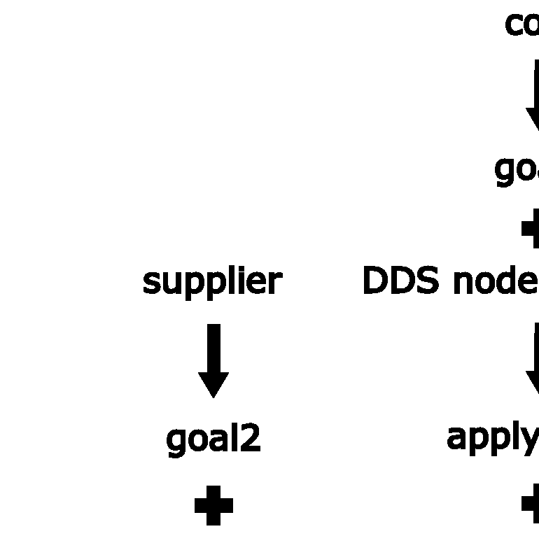
In this lesson, you do not combine the goals at first. You apply node evaluators to the goals individually. You add a search limit to the first goal you execute. In the first phase, you search the search tree with a goal created from the cost variable. You prune the search tree based on a search limit associated with this goal. In the second phase, you search the remaining part of the search tree with a goal created from the supplier variable. In both phases of the search, you use a search selector created from the totalCost variable.

You will perform eight steps to create a final goal to be used in search:

Add the following code after the comment //Create goal1

    IloGoal goal1 = IloGenerate(env, cost, IloChooseMaxRegretMin);

Now, you apply a node evaluator to goal1. In this lesson, you apply a node evaluator that implements Depth-Bounded Discrepancy Search (DDS). DDS makes the assumption that mistakes are more likely near the top of the search tree rather than further down. For this reason, this procedure does not count the number of discrepancies but the depth of the last one.

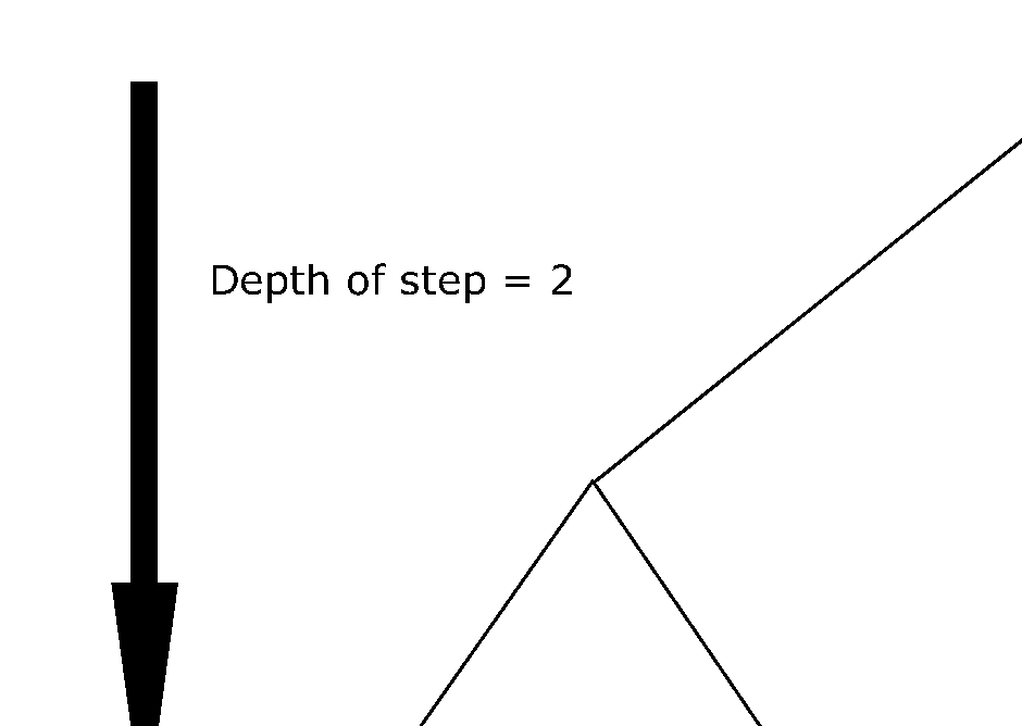
The function IloDDSEvaluator creates and returns an instance of IloNodeEvaluator that implements Depth-Bounded Discrepancy Search. The first parameter is the environment. The second parameter step. Solver will first explore nodes with a depth less than step. After this exploration is complete, it will explore nodes with a depth between step and 2 * step, and so on. The third parameter is width. Solver will look first at paths, starting from the depth level, that have a number of discrepancies, or right moves, less than or equal to width. The fourth parameter is maxDiscrepancy. If this parameter is used, Solver will discard nodes with a number of discrepancies greater than maxDiscrepancy. The default value for maxDiscrepancy is IloIntMax, which means that Solver will not discard any nodes based on this parameter. Here is a constructor:

IloNodeEvaluator IloDDSEvaluator(IloEnv env,
                                 IloInt step = 4,
                                 IloInt width = 2,
                                 IloInt maxDiscrepancy = IloIntMax);

You now use the function IloApply. This function applies the node evaluator IloDDSEvaluator to goal1 and returns applygoal1. The node evaluator will first search paths in the search tree with a depth of 3 or less nodes. It will search paths deeper than this depth that have a number of discrepancies, or right moves, less than or equal to 1.

Add the following code after the comment //Create applygoal1

    IloGoal applygoal1 = IloApply(env, goal1, IloDDSEvaluator(env, 3, 1));

Now, you will apply a search limit to the goal applygoal1. You will use the function IloFailLimit to limit the search after maxNbFails failures have occurred. Here is a constructor:

IloSearchLimit IloFailLimit(IloEnv env, IloInt maxNbFails);

Now, you use the function IloLimitSearch. It takes three parameters: the environment, a goal, and a search limit. This function places a fail limit on applygoal1 and returns limitgoal1. The fail limit stops the search after 5 failures have occurred.

Add the following code after the comment //Create limitgoal1

    IloGoal limitgoal1 = IloLimitSearch(env, applygoal1, IloFailLimit(env, 5));

You use the function IloGenerate to return goal2 for the decision variable supplier.

Add the following code after the comment //Create goal2

    IloGoal goal2 = IloGenerate(env, supplier);

Add the following code after the comment //Create applygoal2

    IloGoal applygoal2 = IloApply(env, goal2, IloSBSEvaluator(env, 1, 1));

Next, you create combinedGoal by joining the following goals with logical AND operators: limitgoal1, applygoal2, and a goal returned by the function IloInstantiate for the variable totalCost.

Add the following code after the comment //Create the combinedGoal

    IloGoal combinedGoal = limitgoal1 && 
                           applygoal2 && 
                           IloInstantiate(env, totalCost);

Then, you create a search selector, minimizeSearchSelector, from the totalCost variable. This search selector stores the leaf of the search tree that represents a solution with the optimal value of the variable totalCost. After the search tree has been completely explored, it reactivates this value. When a solution is found, it adds a constraint that totalCost must be less than or equal to the solution minus 1.

Add the following code after the comment //Create the search selector

    IloSearchSelector minimizeSearchSelector = IloMinimizeVar(env,
                                                              totalCost,
                                                              1);

Finally, you use the function IloSelectSearch. This function takes combinedGoal and minimizeSearchSelector as parameters and returns finalGoal. It applies the search selector minimizeSearchSelector to the goal combinedGoal.

Add the following code after the comment //Create the finalGoal

    IloGoal finalGoal = IloSelectSearch(env,
                                        combinedGoal,
                                        minimizeSearchSelector);

Now, you create an instance of IloSolver to solve the problem expressed in the model. This code is provided for you:

    IloSolver solver(model);

You use the member function IloSolver::solve to search for a solution. You use finalGoal as a parameter of IloSolver::solve.

Add the following code after the comment //Search for a solution

    if (solver.solve(finalGoal))

Compile and run the program. You should get the following results, though the information displayed by IloSolver::printInformation will vary depending on platform, machine, configuration, and so on:

Using default file
30
[[20, 24, 11, 25, 30], [28, 27, 82, 83, 74], [74, 97, 71, 96, 70], [2, 55, 73, 
6
9, 61], [46, 96, 59, 83, 4], [42, 22, 29, 67, 59], [1, 5, 73, 59, 56], [10, 73,
13, 43, 96], [93, 35, 63, 85, 46], [47, 65, 55, 71, 95]]
[1, 4, 2, 1, 3]
------------------------------
Solution:
Store  0 Warehouse:  Rome
Store  1 Warehouse:  Bordeaux
Store  2 Warehouse:  Rome
Store  3 Warehouse:  Bonn
Store  4 Warehouse:  Rome
Store  5 Warehouse:  Bordeaux
Store  6 Warehouse:  Bordeaux
Store  7 Warehouse:  London
Store  8 Warehouse:  Bordeaux
Store  9 Warehouse:  London

Store  0 Cost:  30
Store  1 Cost:  27
Store  2 Cost:  70
Store  3 Cost:  2
Store  4 Cost:  4
Store  5 Cost:  22
Store  6 Cost:  5
Store  7 Cost:  13
Store  8 Cost:  35
Store  9 Cost:  55

Total cost:  383
------------------------------
Number of fails               : 5
Number of choice points       : 10
Number of variables           : 76
Number of constraints         : 76
Reversible stack (bytes)      : 12084
Solver heap (bytes)           : 52284
Solver global heap (bytes)    : 20124
And stack (bytes)             : 4044
Or stack (bytes)              : 4044
Search Stack (bytes)          : 4044
Constraint queue (bytes)      : 11160
Total memory used (bytes)     : 107784
Elapsed time since creation   : 0.02