Solve
 PREVIOUS
NEXT
| IBM ILOG Solver User's Manual > More on Solving > Controlling the Search: Locating Warehouses > Solve |
Solve |
INDEX
 PREVIOUS
NEXT
|
In this lesson, you will learn how to control the search using node evaluators and search selectors. Goals are the mechanism by which Solver implements search strategies. Goals are a bit like building blocks--goals can be created by combining other goals and a function that returns a goal can take other goals as parameters. You will perform five steps to create a final goal:
IloGenerate and IloInstantiate to return three goals, one goal for each of the following decision variables: cost, supplier, and totalCost. Then, you create combinedGoal by joining these three goals with logical AND operators.
SBSNodeEvaluator.
IloApply. This function takes combinedGoal and SBSNodeEvaluator as parameters and returns SBSNodeEvaluatorGoal.
minimizeSearchSelector, using the totalCost decision variable. The objective, which is to minimize the total cost, is treated implicitly by the search selector.
IloSelectSearch. This function takes SBSNodeEvaluatorGoal and minimizeSearchSelector as parameters and returns finalGoal.
The member function IloSolver::solve takes finalGoal as a parameter and searches for a solution. Figure 13.1 demonstrates this procedure.
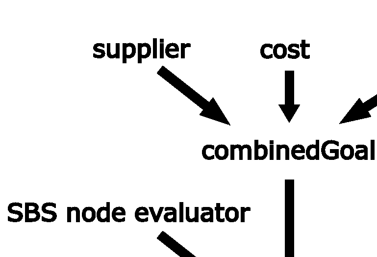
First, you create combinedGoal using logical AND operators. You are already familiar with the predefined goal IloGenerate. The goal IloGenerate takes an array of decision variables as a parameter and calls the function IloInstantiate on each variable in the array. The function IloInstantiate takes a decision variable and binds a value to it.
The first goal binds each decision variable in the array of variables cost using the principle of least regret, or minimizing regret. The IloGenerate parameter IloChooseMaxRegretMin is explained after the following step. The second goal binds each decision variable in the array of variables supplier in the default way, choosing the first unbound variable. The third goal uses the function IloInstantiate to bind the decision variable totalCost.
Step 13 - | Create the combinedGoal |
Add the following code after the comment //Create the combinedGoal
IloGoal combinedGoal = IloGenerate(env, cost, IloChooseMaxRegretMin) && IloGenerate(env, supplier) && IloInstantiate(env, totalCost); |
As you may remember from Chapter 4, Searching with Predefined Goals: Magic Square, the predefined goal IloGenerate allows you to control a choice in the solution search by a parameter which determines which constrained variable Solver tries first. In this lesson, you use the parameter IloChooseMaxRegretMin for the array of variables cost. This parameter uses the principle of least regret to guide the search strategy. Regret is the difference between what would have been the best decision in a scenario and what was the actual decision. In the case of choosing a variable, Solver will select the value for the variable where the difference between the smallest possible value and the next smallest value is maximal.
The following table shows the relative supply costs for the stores. The best decision for each individual store is the warehouse with the lowest relative cost. The second best decision is the warehouse with the second lowest relative cost. The lowest and second lowest costs are in bold.
To illustrate the principle of least regret, examine one small decision. The supplier warehouse located in Bonn has a capacity of one store. Which store should be supplied by the warehouse in Bonn? Two likely candidates are store 3, with a relative cost of 2, and store 6, with a relative cost of 1. If you just looked at this information, you would likely make the decision to use the Bonn warehouse to supply store 6, since the relative cost is lower. However, choosing the Bonn warehouse to supply store 6 will force store 3 to be supplied by the Bordeaux warehouse, with the next lowest relative cost for store 3. You can also imagine what would happen if you choose the Bonn warehouse to supply store 3 and forced store 6 to be supplied by the Bordeaux warehouse, with the next lowest relative cost for store 6. Take a closer look at the two scenarios.
Scenario A |
Warehouse |
Relative Cost |
|---|---|---|
store6 |
Bonn |
1 |
store3 |
Bordeaux |
55 |
Total cost Scenario A |
56 |
Scenario B |
Warehouse |
Relative Cost |
|---|---|---|
store6 |
Bordeaux |
2 |
store3 |
Bonn |
5 |
Total cost Scenario B |
7 |
You can see that Scenario B is a much better choice for the total cost, even though the original choice to supply store 3 from the Bonn warehouse rather than store 6 is a slightly more costly decision than its inverse. You can use the principle of least regret to make just this kind of decision. If you had examined the difference between the lowest relative cost and the next lowest relative cost for store 3, you would see that it is 53. The difference for store 6 is only 4. In deciding which store to supply from Bonn, choose the store with the largest difference. This decision will give you the lowest total cost and cause the least regret.
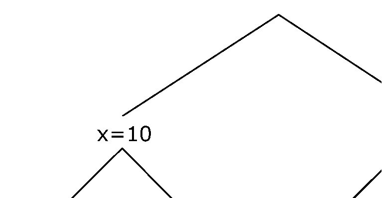
Now that you have created combinedGoal, you create a node evaluator and a search selector. Before you can do this, you need to learn more about search trees, nodes, and selectors. As you remember from Chapter 1, Constraint Programming with IBM ILOG Solver, the search tree is the part of the search space remaining after initial constraint propagation. In the search tree, Solver will use a search strategy to search for a solution. Chapter 1, Constraint Programming with IBM ILOG Solver contained many diagrams of the search tree to help you visualize the search process. These diagrams were simplified versions of the search tree. Solver actually performs a binarization of the search tree, representing every choice as a binary decision. Figure 13.2 is a binary representation of the search tree originally shown in Figure 1.2. As you can see in Figure 13.2, every decision is a binary one. For example, if Solver selects the value 10 for variable x, there are now two choices. Solver can either try the value 5 for variable y or choose not to try value 5 for variable y. If Solver chooses not to try value 5 for variable y, Solver is again confronted with two choices. Solver can now either try the value 6 for variable y or the value 7 for variable y.
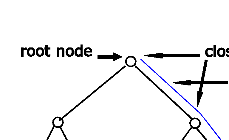
A search tree is composed of nodes connected by branches. The root of the tree is the starting point in the search for a solution; each branch descending from the root represents a decision in the search. At the beginning of the search, all the nodes in the tree are unexplored nodes. Solver starts the search at the root node. At this point, the root node is called an open node, since no decision has yet been made. There are two possible decisions to make at this open node--these two possible decisions are called leaves. Solver selects a leaf. The root node is now a closed node, since a decision has been made. The selected leaf is now a branch and the node at the other end of this branch is now the open node. Two leaves come off this open node, representing two possible decisions. Tree traversal is the technique used to explore the search tree. As Solver traverses a search tree, it builds an active path. Each node, except for the terminal ones, has one or more child nodes and is called the parent of its child nodes. Removing branches from the search tree is pruning. Node evaluators guide how Solver traverses the search tree--which nodes are evaluated and in what order. Search selectors determine how Solver makes decisions at open nodes--a search selector guides the selection of a leaf.
These concepts are shown in Figure 13.3.
As a default, Solver uses Depth-First Search (DFS) to traverse the search tree and control the order of node evaluation--Depth-First Search is the default node evaluator. Depth-First Search explores the search tree in a "left-to-right" fashion. It searches by selecting the left leaf at each open node until the end of the search space is reached. If it does not find a solution, it backtracks and tries again. Figure 13.4 shows tree traversal using Depth-First Search (DFS). The numbers at the bottom represent the order in which paths are created by the search strategy.

Depth-First Search is a straightforward approach to searching for a solution. However, sometimes you may have some knowledge about the search tree--you may know that certain parts of the search tree are more likely to contain a solution. In this case, you may want to change the order of node evaluation, since you think that certain nodes are more likely to lead to a solution. To do this, you can use a different node evaluator. There are several predefined functions in Solver that create and return node evaluators. To learn more about them, see Chapter 12. In this lesson, you will use the predefined function IloSBSEvaluator to create and return a node evaluator based on the principle of Slice-Based Search (SBS).
Usually, you have some kind of strategy to solve your problem. Therefore, you hope that Solver will not make many mistakes as it searches for a solution. In search trees, right moves are considered mistakes and left moves are considered correct decisions. So, if you think you have a good search strategy, it would make sense to look for a solution first among the nodes in paths that have fewer right moves. By searching first among the paths with fewer right moves you are saying you believe in your search strategy and you are trying to stick to it.
Slice-Based Search (SBS) does this. It looks first in the paths of the tree with fewer right moves. A right move in the path from the root of the search tree to the current node is known as a discrepancy. By looking first in paths with fewer right moves, Slice-Based Search cuts the search tree in slices.
The function IloSBSEvaluator creates and returns an instance of IloNodeEvaluator that implements Slice-Based Search. The first parameter is the environment. The second parameter is step. Solver will look first at paths that have a number of discrepancies, or right moves, less than or equal to step. The third parameter is maxDiscrepancy. If this parameter is used, Solver will discard nodes with a number of discrepancies greater than maxDiscrepancy. The default value for maxDiscrepancy is IloIntMax, which means that Solver will not discard any nodes based on this parameter. Here is a constructor for IloSBSEvaluator
IloNodeEvaluator IloSBSEvaluator(IloEnv env, IloInt step = 4, IloInt maxDiscrepancy = IloIntMax); |
Figure 13.5 shows a search tree that has been traversed with a node evaluator using Slice-Based Search with a discrepancy of 1. The numbers in row 1 represent the order in which paths are evaluated. As you can see, Solver searches in slices as opposed to the "left-to-right" strategy of Depth-First Search (DFS). Solver first evaluates paths 1, 2, and 3. It then jumps to path 4 and then jumps again to path 5. It jumps back to path 6 and so on. The numbers in row 2 represent the number of discrepancies, or right moves, in each path. As you can see, Solver first search the paths with 0 or 1 discrepancy, then the paths with 2 discrepancies, then the paths with 3 discrepancies, and finally the path with 4 discrepancies.

Now that you understand the concepts behind node evaluators, you can create one. The node evaluator SBSNodeEvaluator will first search paths in the search tree with 4 or less discrepancies.
Step 14 - | Create the node evaluator |
Add the following code after the comment //Create the node evaluator
IloNodeEvaluator SBSNodeEvaluator = IloSBSEvaluator(env, 4); |
Now that you have created the node evaluator, you need to apply it to combinedGoal, the goal you created in Step 13. To do this you use the function IloApply. This function takes combinedGoal and SBSNodeEvaluator as parameters and returns SBSNodeEvaluatorGoal. It applies the node evaluator SBSNodeEvaluator to the goal combinedGoal.
Step 15 - | Create the SBSNodeEvaluatorGoal |
Add the following code after the comment //Create the SBSNodeEvaluatorGoal
IloGoal SBSNodeEvaluatorGoal = IloApply(env, combinedGoal, SBSNodeEvaluator); |
Now that you have created and applied a node evaluator, you create a search selector. This search selector will guide the search at each open node. In this problem, you want to select the leaf at each open node that will minimize the total cost of the solution. To do this, you use the function IloMinimizeVar. This function returns an instance of the class IloSearchSelector. It takes three parameters: the environment, the variable to be minimized, and a step. Here is a constructor:
IloSearchSelector IloMinimizeVar(IloEnv env, IloNumVar var, IloNum step = 0); |
The search selector IloMinimizeVar does several things:
var--in this example, the solution with the lowest totalCost. After the search tree has been completely explored, it reactivates this value. In other words, it stores the leaf representing the current best solution and gives the search the ability to go back to that leaf if it does not find a better solution.
var must be less than or equal to the solution minus step. For example, if the search selector (with step = 0.1) finds a solution with totalCost equal to 300, it adds a constraint that totalCost must be less than or equal to 300 - 0.1 or 299.9 for the remainder of the search.
Step 16 - | Create the search selector |
Add the following code after the comment //Create the search selector
IloSearchSelector minimizeSearchSelector = IloMinimizeVar(env, totalCost, 0.1); |
Now that you have created the search selector minimizeSearchSelector, you need to apply it to SBSNodeEvaluatorGoal, the goal you created in Step 15. To do this, you use the function IloSelectSearch. This function takes SBSNodeEvaluatorGoal and minimizeSearchSelector as parameters and returns finalGoal. It applies the search selector minimizeSearchSelector to the goal SBSNodeEvaluatorGoal.
Step 17 - | Create the finalGoal |
Add the following code after the comment //Create the finalGoal
IloGoal finalGoal = IloSelectSearch(env, SBSNodeEvaluatorGoal, minimizeSearchSelector); |
Now, you create an instance of IloSolver to solve the problem expressed in the model. This code is provided for you:
IloSolver solver(model); |
You now use the member function IloSolver::solve to search for a solution. In this lesson, you use finalGoal as a parameter of IloSolver::solve.
Step 18 - | Search for a solution |
Add the following code after the comment //Search for a solution
if (solver.solve(finalGoal)) |
The member functions and streams IloAlgorithm::out and IloSolver::getValue are used to display the solution. When you print the solution, you associate the value for the supplier warehouse variable supplier with the warehouse location using the array Suppliers[], which is provided for you in the exercise code. The following code is provided for you:
Step 19 - | Compile and run the program |
Compile and run the program. You should get the following results, though the information displayed by IloSolver::printInformation will vary depending on platform, machine, configuration, and so on:
As you can see, the solution uses four warehouse sites: Bonn, Bordeaux, London, and Rome. All stores are supplied by a supplier warehouse and the total cost is 383.
The complete program is listed in "Complete program". You can also view it online in the file YourSolverHome/examples/src/storesbs.cpp.
| © Copyright IBM Corp. 1987, 2009. Legal terms. | PREVIOUS NEXT |