Defining the Problem, Designing a Model
 PREVIOUS
NEXT
| IBM ILOG Scheduler User's Manual > Advanced Concepts > Using Strong Propagation on Reservoirs: the Balance Constraint > Defining the Problem, Designing a Model |
Defining the Problem, Designing a Model |
INDEX
 PREVIOUS
NEXT
|
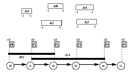
Suppose we introduce a set of time variables t0, ..., tn such that ti is constrained to execute between the end of the activity ranked at position i-1 and the start of the activity ranked at position i as described in Figure 22.1.
The constraint C(i, j, d) can be expressed by (tj - ti >= d). Of course, the problem is that one doesn't know the actual activity that is ranked at position i until the activities have been ranked. Therefore, we have to implicitly constrain the time points ti to be between the activity ranked at position i-1 and the one ranked at position i. This can easily be done with an additional resource that is a reservoir of capacity 2 and initial level 0. Each real activity ak on the unary resource will consume 1 unit of this reservoir at its start time and consume 1 unit of reservoir at its end time. We introduce a chain of n fake activities, pi, that produce 2 units of reservoir at their start time ti. The duration of these fake activities is chosen to be 1 but it could be any duration. The chain of fake activities is defined by taking ti < tj. This model is shown in Figure 22.2.

We see that, due to the minimal and maximal level on the reservoir, between ti and ti+1 there must be at least two resource consumptions. Because of the unary resource, we also see that these two resource consumptions must correspond to the start of an activity ak followed by its end. Thus ti, the start time of pi, is really a time-point between the activity ranked at position i-1 and the one ranked at position i. We can post the constraints (tj - ti >= d) directly as temporal constraints between the fake activities pi on the reservoir.
The model is implemented as follows. As usual, a function creates and returns the model:
IloModel DefineModel(const IloEnv& env, IloInt numberOfActivities, IloInt numberOfConstraints, IloInt* durations, IloInt* constraints, IloNumVar& makespan) { IloModel model(env); |
First of all, an upper bound of the optimal makespan is computed and used to define the range of the makespan variable. This upper bound is computed as follows: suppose that there exists an optimal solution Sopt, that is, a total order between the activities ak (similar to the one described on Figure 22.1) that satisfies the temporal constraints between the time points ti. For simplicity, we assume Sopt = (a0, a1, ..., an-1). It's easy to show that the optimal makespan corresponding to this total order is the minimal value of tn that satisfies:
In other words, given a feasible total order, the optimal makespan can be easily computed simply by propagating the PERT associated with the schedule and is equal to the minimal value of tn after propagation. If we use a more pessimistic version of this PERT where all activities have the same duration, that is, the one of the longest activity ak, we will obtain a worse makespan. This makespan, however, will be an upper bound of the optimal makespan obtained for any total order between activities. That's the idea of the function getMakespanMax below.
  IloNum makespanMax = getMakespanMax(env,
                                      numberOfActivities,
                                      numberOfConstraints,
                                      durations,
                                      constraints);
  makespan = IloNumVar(env, 0, makespanMax, ILOINT);

IloNum getMakespanMax(const IloEnv& env,
                      IloInt numberOfActivities,
                      IloInt numberOfConstraints,
                      IloInt* durations,
                      IloInt* constraints) {
  // THIS FUNCTION COMPUTES AN UPPER BOUND ON THE MAKESPAN BY ASSUMING
  // ALL THE ACTIVITIES HAVE A  DURATION EQUAL TO THE LONGEST ACTIVITY
  // OF THE   PROBLEM.
  IloModel model(env);

  IloNumVar makespan(env, 0, IloInfinity, ILOINT);
  IloInt i, j, k, t;

  // COMPUTE MAXIMAL DURATION OF ACTIVITIES
  IloInt dmax = 0;
  for (i=0; i < numberOfActivities; i++)
    if (durations[i] > dmax)
      dmax = durations[i];

  IloActivity lact;
  IloNumExprArray times(env, numberOfActivities+1);
  for (i=0; i < numberOfActivities; i++) {
    // USE ACTIVITIES WITH MAXIMAL DURATION
    IloActivity act(env, dmax);
    times[i] = act.getStartExpr();
    if (i > 0)
      model.add(act.startsAfterEnd(lact));
    lact = act;
  }
  model.add(lact.endsBefore(makespan));
  times[numberOfActivities] = makespan;

  // ADD MINIMAL DELAY CONSTRAINTS
  for (k=0; k < numberOfConstraints; k++) {
    i = constraints[3*k];
    j = constraints[(3*k) + 1];
    t = constraints[(3*k) + 2];
    model.add(times[j]-times[i] >= t);
  }

  // JUST PROPAGATE THE PERT
  IloSolver solver(model);
  IlcSearch s = solver.newSearch(IloGoalTrue(env));
  s.next();
  IloNum makespanMax = solver.getMin(makespan);
  solver.end();

  return makespanMax;
}
Now that the range of the makespan variable has been defined, we need to define the main ingredients of the model itself. As mentioned above, we need to define two resources: the unary resource that will impose a total order between the activities ak and the reservoir that will implicitly constrain the time points ti to be in between the activities ak.
In this scheduling problem, we see that our primary reasoning concerns the relative position of activities rather than the absolute dates at which activities execute. As we noticed before, once a total order between activities ak has been found, computing the corresponding optimal makespan is easy. Thus, the main problem is finding an optimal total order and we need to use propagation algorithms that perform strong pruning of the search by analyzing the relative positions of activities.
On the reservoir, we will post a balance constraint. This constraint is described in Balance Constraint in the IBM ILOG Scheduler Reference Manual. The balance constraint internally maintains a precedence graph between the time points (start, end) of the activities on the resource. It propagates by analyzing this graph in order to discover new time bounds for activities as well as new precedence relations between activity time points. In the Concert Technology model, the balance constraint is specified by the level IloExtended for the capacity enforcement as described in Resource Enforcement as Global Constraint Declaration in the IBM ILOG Scheduler Reference Manual.
IloReservoir reserv(env, 2, 0); // THIS ENFORCEMENT LEVEL WILL POST THE BALANCE CONSTRAINT reserv.setCapacityEnforcement(IloExtended); |
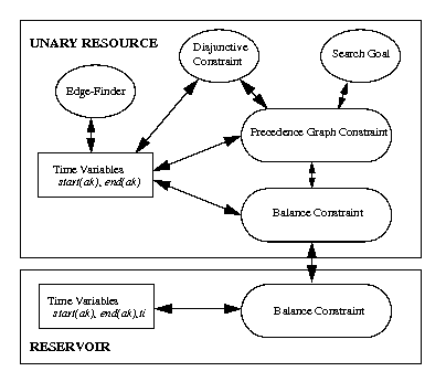
On the unary resource we will also post a balance constraint as well as a precedence graph constraint. The precedence graph constraint will collect all the new precedences detected by the disjunctive constraint and the edge-finder on the unary resource as well as the rank information on activities. The balance constraint on the unary resource will get this precedence information from the precedence graph and also exchange information with the balance constraint of the reservoir.
This combination of global constraints ensures that whenever a total order between activities ak on the unary resource has been found, the balance constraint on the reservoir knows that the set of reservoir consumption (at the start and end of activities ak) is totally ordered and this implies that the fake reservoir productions at time points ti are correctly interleaved between the activities ak. Thus, it ensures the soundness of the search, even though the search goal IloRankForward (see Solving the Problem) does not completely instantiate the start and end times of activities. Of course, during the search, the balance constraint on the reservoir may discover new precedence relations between activities. These precedence relations are automatically inserted in the unary resource precedence graph via the balance constraint of the unary resource and they enable reduction of the search tree by removing some possibly first resource constraint on the unary resource. The global communication between constraints is illustrated on Figure 22.3.

The rest of the definition of the model creates the activities and the resource constraints. Note how some evident symmetries of the problem are broken by ordering the subsets of activities of the same duration before solving. Note also that a delay dmin corresponding to the minimal duration of activities is inserted between each time point ti.
  IloNumExprArray times(env, numberOfActivities + 1);
  IloActivityArray acts(env, numberOfActivities);

  // COMPUTE DURATION OF SHORTEST ACTIVITY
  IloInt dmin = IloIntMax;
  IloInt i, j, k, t;
  for (i=0; i < numberOfActivities; i++)
    if (durations[i] < dmin)
      dmin = durations[i];

  IloActivity lprod;
  for (i=0; i < numberOfActivities; i++) {
    acts[i]= IloActivity(env, durations[i]);
    model.add(acts[i].requires(ures));
    model.add(acts[i].requires(reserv, 1, IloAfterEnd));
    model.add(acts[i].requires(reserv, 1, IloAfterStart));
    model.add(acts[i].endsBefore(makespan));
    IloActivity prod(env, 1);
    model.add(prod.provides(reserv, 2, IloAfterStart));
    times[i] = prod.getStartExpr();
    if (i > 0)
      // BUILD CHAIN OF PRODUCERS
      model.add(prod.startsAfterStart(lprod, dmin));
    lprod = prod;
  }
  times[numberOfActivities] = makespan;
  model.add(times[numberOfActivities-1] + dmin <= makespan);

  // BREAK EVIDENT SYMMETRIES BETWEEN ACTIVITIES WITH SAME DURATION
  for (i=0; i < numberOfActivities - 1; i++)
    for (j=i+1; j < numberOfActivities; j++)
      if (durations[i] == durations[j]) {
        model.add(acts[j].startsAfterEnd(acts[i]));
        break;
      }

  // ADD DELAY CONSTRAINTS
  for (k=0; k < numberOfConstraints; k++) {
    i = constraints[3*k];
    j = constraints[(3*k) + 1];
    t = constraints[(3*k) + 2];
    model.add(times[j]-times[i] >= t);
  }

  return model;
| © Copyright IBM Corp. 1987, 2009. Legal terms. | PREVIOUS NEXT |