Tutorial: Tuning the Propagation in the debuggolomb Example

IBM ILOG Solver Debugger User's Manual > Debugging and Performance Tuning for Solver-based Applications > Improving your Application > Tutorial: Tuning the Propagation in the debuggolomb Example

Tutorial: Tuning the Propagation in the debuggolomb Example

INDEX

PREVIOUS NEXT

This section is based on the debuggolomb example. It shows you how Solver Debugger can be used to tune the propagation of a Solver application.

Filter levels

In order to tune the propagation in the debuggolomb example, we will use the alldiff global constraint of Solver with two different levels of propagation.

Reminder

When connecting to the debuggolomb example, pass two integer parameters: the size of the problem and the filtering level of the alldiff constraint.

debuggolomb 6 0 (0 = basic filtering level)

debuggolomb 6 1 (1 = medium filtering level)

debuggolomb 6 2 (2 = extended filtering level)

When using the basic filter level of this constraint, Solver guarantees that, at any computation point, the specified variables do not have the values of the already-assigned variables inside their domain.
When using the extended filter level, Solver reasons on the domains instead of the values and guarantees that, for each value in the domain of any given variable, there exist values in the domains of the remaining variables such that the constraint is satisfied.

Using the Search Tree

Visualize the Search Trees corresponding to the basic and extended filter levels. The following figure represents the Search Trees corresponding to the two filter levels.

In the Search Tree, the extended level enforces a stronger pruning than the basic one, while the basic filter level produces a bigger tree with additional right subtrees.

These right subtrees have only failure leaves, which is a sign of lack of propagation. By setting the filter level to the extended level these right subtrees are pruned.

Using the Christmas Tree

The Christmas Tree provides a picture of the cost and the efficiency of the extended propagation.

Compare the number of propagation events in the first right subtree located in the frame in Figure 1.6 with the number of propagation events occurring at the corresponding big failure node in Figure 1.7.

Figure 1.6 The Christmas Tree for the debuggolomb problem with a basic level of propagation

Figure 1.7 The Christmas Tree for the debuggolomb problem with an extended level of propagation

The big node requires two times fewer propagation events to detect the failure than the subtree. So the extended propagation saved time.

Now compare the Initial Propagation statistics by looking at the root node. The efficiency of domain reduction is the same (63.25%).

Using the Propagation Spy

Inspect the Initial Propagation. Solver adds a hidden constraint when posting the alldiff constraint. When tracing the propagation at the first big failure node of the extended filter level, the Propagation Spy displays the extra propagation, as shown in the figure below.

Figure 1.6 Comparing two propagation traces using the Propagation Spy for the debuggolomb problem

With the basic filter level, the propagation stops after reducing the variable difference[11] to the interval [7..11].
With the extended level, the propagation of an additional internal constraint posted by the alldiff constraint strongly reduces the domains by means of Set Min events. This additional propagation leads to a failure, avoiding a subtree exploration.

Notice that four Set Min events are triggered on the difference[11] variable where one should be enough. These Set Min events are Remove Value orders that have been translated by Solver into Set Min because the value to remove was a bound.

So, reasoning on bounds instead of on domains is sufficient in this case. Tune the alldiff constraint to the intermediate filter level, which reasons on bounds instead of on domains.

You obtain the same Search Tree as with the extended filter level. The Propagation Spy shows that, at the same choice point, the variable difference[11] is bound more quickly.

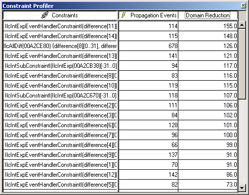
Figure 1.9 Propagation Spy for the debuggolomb problem with an intermediate filter level

Using the Constraint Profiler

You can paste the matrix from the Constraint Profiler to Microsoft Excel and make your own statistics. For instance, summing the propagation events gives the results shown below. The table contains the statistics on the number of events for the debuggolomb problem.

Filter Level	Total Number of Events
Basic	3534
Intermediate	2726
Extended	2790

PREVIOUS NEXT