RSSI fluctuations due to signal noise significantly affect both stability and efficiency. For instance, in HP communication-level
handover, when the RSSI value of the current AP is slightly greater than the sum of another AP RSSI plus HHT, even small RSSI
fluctuations can produce several Prob changes, thus relevantly reducing stability. In addition, in those conditions RSSI
over/underestimation may trigger unnecessary predictions, thus lowering efficiency.
In this section we specifically analyse, and quantitatively compare different techniques (Grey Model,
Fourier Transform, Discrete Kalman, and Particle) for filtering RSSI fluctuations due to signal noise, by pointing out how
filtering can positively impact on handover/mobility prediction performance.
Grey Model
We have designed and implemented a first-order Grey Model filtering module that calculates filtered RSSI values on the basis of a finite series of RSSI values monitored in the recent past. In particular, given one visible AP and the set of its actual RSSI values measured at the client side R0 = {r0(1), …, r0(n)}, where r0(i) is the RSSI value at the discrete time i, it is possible to calculate R1 = {r1(1), …, r1(n)}, where: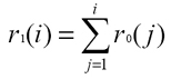
Then, from the Grey Model discrete differential equation of the first order:
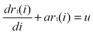
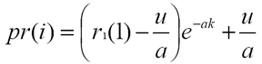
the wireless client can autonomously determine a and u, which are exploited to obtain the predicted RSSI value pr(i) at discrete time i according to the Grey Model prediction function:
Let us observe that filtered RSSI depends on the number of actual RSSI values r0(i) employed in the Grey Model. In principle, longer the finite input series R0, more regular the RSSI filtered values, and slower the filtered RSSI sequence follows the possibly abrupt time evolution of actual RSSI. We have experimentally evaluated the Grey Model performance while varying the R0 size; the best trade-off between RSSI fluctuation mitigation and actual-to-filtered RSSI delay is usually for R0 size=15 and we used this value to obtain the reported experimental results.
Fourier Transform
Our Discrete Fourier Transform (DFT) filtering module extract from R0 a Fourier coefficient set (Ai and Bi) representing the RSSI sequence in the frequency domain in the time window R0 size*RSSI sample interval. The coefficient set is extracted with the usual Fourier equations:
The Fourier coefficient set is the basis to define an Inverse Discrete Fourier Transform (IDFT) to regenerate the RSSI signal:

When IDFT exploits only a subset of the above series terms, the regenerated RSSI sequence do not exhibit its high frequency components and shows a more regular trend, i.e., IDFT behaves as a low pass filter. We have tested our Fourier Transform filter with several values for R0 size and number of addends: we have found a good trade-off between fluctuation mitigation and actual-to-filtered delay with R0 including 4 values and IDFT only its first term.
Discrete Kalman
Our Discrete Kalman filtering module tries to est i-mate RSSI values by representing the RSSI time evolution as a combination of signal noise (measurement noise) and maximum signal evolving (process noise). A linear stochastic equation models the RSSI evolution, with signal/process noise assumed to be independent of each other, white, and with normal probability distribution (standard deviation Q/R).Our filter works by minimizing process/measurement noise through a two phase algorithm: first, a predictor performs next RSSI estimation; then, a corrector improves RSSI estimation by exploiting current RSSI measurement. Therefore, an iteration of our Discrete Kalman filtering module processes:

where P(k) is the covariance matrix of the state estimate error, with initial value Q, and K(k) is usually indicated as the Kalman Gain in the filtering literature.
In our scenario x and z are RSSI values, the state coincides with the output (A is a 1x1 identity matrix), and the estimation of the next state estimate is equal to the current state (H is a 1x1 identity matrix). After several tests, we have found a good trade-off between RSSI fluctuation mitigation and filtered-to-actual RSSI delay by setting Q=1.6 and R=6.
Particle
Like Discrete Kalman, our Particle filtering module tries to estimate RSSI by minimizing measurement and process noise, but without imposing a linear equation modeling and, more important in our deployment scenario, without imposing normal distribution for signal noise. The main idea at its basis is to have an algorithm that computes, at each step, several possible filtered RSSI values for each measured RSSI; then, the filter associates each candidate value with a weight and chooses the most promising values among them when a new measured RSSI is available; finally, it perturbs candidate values, according to the rules shown below, thus obtaining a new filtered RSSI (the average value of the most promising candidates). To better and practically understand how Particle Filter works, let us show a rapid example of algorithm iteration with 10 particles, which represents 10 possible filtered RSSI values (Figure 2):- starting step - there are 10 possible filtered RSSI values (light circles), all with the same weight;
- importance weight step - by exploiting state est i-mate probability (black curve) obtained from RSSI measurement, the algorithm assigns a weight at each filtered RSSI value (dark circles);
- re-sampling step - heavy RSSI are spread in different RSSI values, all with the same weight (light circles), while light RSSI values are discarded;
- sampling/prediction step - filtered RSSI are randomly perturbed (light circles).

Figure 1. An example of Particle iteration.
The number of particles strongly influences the Particle filter performance; in general greater is the particle number, better the filtered RSSI follows the actual RSSI sequence. Differently from the previous 3 filters, Particle has a non-negligible computational load, which deeply depends on the particle number. Table 1 shows one iteration time by exploiting a High Capability machine (an Intel Pentium4 2.80GHz, 1024 MB of RAM) and a Low Capability one (mobile AMD Athlon 2000+ 1.66 GHz, 480 MB of RAM). For example one iteration of our Particle filter, High Capability machine, takes about 132ms with 250 particles and 521ms with 500 particles; in a practical deployment scenario, where multiple APs are simultaneously visible from wireless clients, that time should be multiplied by the number of visible APs, and the computation occurs at any sampling interval. For the sake of completeness, we will report also Particle performance, when used with 250 particles and with the same Q and R are as in Discrete Kalman; however, current client-side resource limitations discourage the exploitation of the Particle filtering module.
|
 |
|---|
A Rapid Preliminary Comparison of RSSI Filtering Modules
Just to give a preliminary rough comparison of the behaviors of the proposed filters, Figure 3 reports 60 RSSI samples, either actually measured or filtered ac-cording to one of the 4 filtering modules. In particular, the figure points out how much filters are able to mitigate RSSI fluctuations and how fast filtered RSSI sequences follow the actual ones in the case of rapid RSSI evolving, e.g., samples 5 and 45.Figure 2 is exemplar of the actual RSSI strong fluctuations (filter = Identity). Compared to actual RSSI, the output of the Grey Model has definitely less fluctuations, but tends to overestimate and to amplify RSSI growth in the case of rapid increasing, for instance when wireless clients are very close to their APs (see samples 10 and 50). Fourier and Kalman have similar behaviors: both tend to mitigate RSSI fluctuations quite well and accurately follow the actual RSSI sequence, without overestimating RSSI changes. Particle mitigates RSSI fluctuations very well, but sometimes introduces a non-negligible delay between actual and filtered values (see samples 8 and 47).
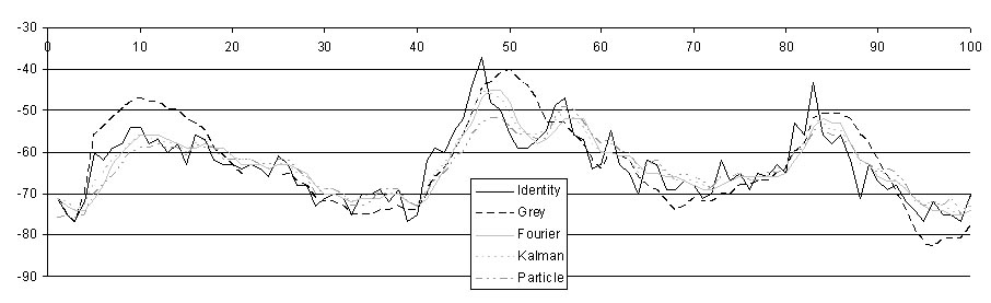
Figure 2. Actual and filtered RSSI.
Experimental Results
We report experimental results about the different hit rate, efficiency, and stability performance achieved when feeding our Prob module either with actual RSSI data or filtered RSSI (exploiting each time one of the 4 proposed filters). As already stated, the primary goal of RSSI filtering in our proposal is to mitigate RSSI fluctuations due to signal noise in order to primarily improve hit rate, with simultaneous acceptable values for efficiency and stability. However, better a filter mitigates RSSI fluctuations and longer is filtered-to-actual RSSI delay; in the following, for each filter we have adopted the parameter tuning described above, which achieves a suitable trade-off between introduced delay and filtering performance.In particular, in the case of handover prediction we have defined the following performance indicators:
hit rate |
 |
where HPpre is the total time elapsed in HighProb state in the t-long interval before handover
and HPopt is the time an optimal predictor should stay in HighProb state (exactly t seconds before each
handover). We have chosen t=4s because such a time interval is largely sufficient to perform the needed service management
operations in the WI localities going to be visited |
|---|---|---|
efficiency |

|
where HPtot is the total time elapsed in HighProb state |
stability |
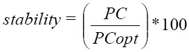 |
where PC is the number of Prob state changes of our predictor and PCopt the optimal number of
Prob state changes |
On the contrary, in the case of mobility prediction, we are interested in evaluating:
hit rate |
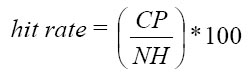
|
where CP is the number of correctly predicted handovers and NH is the total number of performed handovers |
|---|---|---|
efficiency |
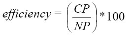 |
where NP is the total number of triggered predictions |
Obviously, efficiency and hit rate are strongly correlated: on the one hand, very good values for hit rate can be achieved at the expense of poor efficiency values; on the other hand, it is possible to obtain very good efficiency by simply delaying as much as possible handover predictions, with the risk of missing handovers (too low hit rate). Moreover, it is necessary to maintain sufficiently high stability not to continuously perturb the service infrastructure with useless and expensive management operations.
We have measured the five indicators above in a challenging simulated environment, with a large number of Wi-Fi clients roaming among a large number of wireless APs (17 APs regularly deployed in a hexagonal cell topology); RSSI fluctuation has a 3dB standard deviation, FPT=72dB, FHT=80dB, HPT=2dB, HHT=6dB. Wireless clients follow movement trajectories according to either i) the usual Random Waypoint model, speed is in the range [0.6m/s, 1.5m/s] and "thinking time" between 0s and 10s", or ii) our proposed Continuous model.
We have compared the behavior of the 4 proposed filtering modules within 12 scenarios (about 200 handovers performed in each one), differentiated for AP to AP distance (20m, 30m or 40m), type of communication-level handover (HP or SP) and wireless client mobility model (waypoint vs. continuous). First of all we consider only the scenarios with dense AP and waypoint mobility model, then we describe differences between those and other scenarios.
Figures 3-7 reports average values of performance indicators for handover and mobility prediction, in various scenarios with different AP density, wireless client mobility model and handover strategy. Table 2 explains some acronyms.
Mobility Model |
W | Random Waypoint model | C | Continuous model | ||||
Handover Strategy |
HP | Hard Proactive handover strategy | SP | Soft Proactive handover strategy | ||||
AP density |
Ld | AP Low density (40m AP-to-AP distance) | Md | AP Medium density (30m AP-to-AP distance) | Hd | AP High density (20m AP-to-AP distance) |
In general, the adoption of the proposed filtering techniques significantly improves Handover Prediction stability, with relevant benefits from the point of view of system overhead due to useless Prob state changes. Efficiency also increases when exploiting filtered RSSI, except than in the case of Grey Model: in fact, Grey Model filtering tends to amplify the growth/decreasing trends of actual RSSI values, as observed in the previous section; that produces handover/mobility predictions with a large advance time but also with limited efficiency. Fourier, Kalman, and Particle filters, instead, tend to delay a little more Prob state changes, thus increasing efficiency. Let us observe that the hit rate performance indicator slightly decreases when adopting filtering techniques, except than in the Grey Model case. That effect is tied to what observed before: a slightly greater delay in handover prediction tends to weakly worsen hit rate, but with the relevant advantage of a significantly greater stability.
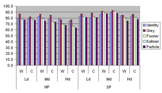
Figure 3. Handover Prediction Hit Rate.

Figure 4. Handover Prediction Efficacy.

Figure 5. Handover Prediction Stability.

Figure 6. Mobility Prediction Hit Rate.
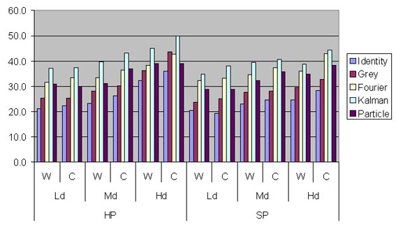
Figure 7. Mobility Prediction Efficacy.
By taking a look at the whole set of reported performance results, it is clear that there is not a filtering technique always outperforming the others. Filtering exploitation has demonstrated to be crucial for increasing stability; the decision on which filter to exploit depends on the specific goals of the provisioned mobile service. On the one hand, if it is of key relevance to achieve very high hit rates, the Grey Model is to be considered. On the other hand, if prediction costs must be as low as possible (high efficiency), Fourier and Kalman are good candidates. Let us stress that, thanks to the modular architecture of our middleware, it is possible to choose the exploited filtering module at provisioning time, by adapting middleware behavior to the current service context. For instance, consider the case that our middleware exploits handover prediction to support the pre-fetching of data chunks before handover, in order to continuously provide service flows also during AP changes with temporary disconnections. If the crucial point is to avoid temporary service interruptions, the best choice is Grey Model filtering; otherwise, if the priority is to minimize useless exploitation of client-side buffers, either Fourier or Kalman should be chosen. Finally, as already stated, Particle should be excluded from possible choices be-cause of its high client-side computational load.