Tracking Application |
In the Main Page
we sketched some application cases for MobEyes. For the
sake of proving its effectiveness in supporting urban monitoring, we
also simulated a vehicle tracking application where the agent reconstructs node
trajectories exploiting the collected summaries. This is a challenging application,
since it requires our system (1) to monitor a large number of targets, i.e., all participant vehicles,
(2) to periodically generate fresh information on these targets, since they
are highly mobile, (3) to deliver to the agent a high share of the generated information.
Moreover, since nodes are generally spread all over the area, this application
shows that a single agent can maintain a consistent view of a large zone of responsibility.
More in details, as regular cars move in the field, they generate new summaries
every T=120s and continuously advertise the last generated summary.
Every summary contains
60 summary chunks, which are created every ChunkPeriod=2s
and include the license plate and position of the vehicle
nearest to the summary sender at the generating time, tagged with a timestamp.
The application exploits the MobEyes diffusion protocol with k=1 to spread
the summaries and deliver as much information as possible to a single agent
scouting the ground. As the agent receives the summaries, it extracts the information
about node plates and positions, and tries to reconstruct node trajectories within the area.
This is possible by aggregating data related to the same license plate, reported
from different summaries.
To determine the effectiveness of MobEyes we decided to evaluate the average uncovered
interval and maximum uncovered
interval for each node in the field. Given a set of summary chunks related to the
same vehicle and ordered on time basis, these parameters measure respectively
the average period for which the agent does not have any record for that vehicle
and the longest period. The latter typically represents situations in which
a node moves in a zone where vehicle density is low; thus, it cannot
be traced by any other participant.
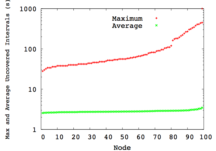
We associated the average and maximum uncovered intervals to each simulated node, and
present the results in next Figure (note the logarithmic scale on the Y-axis).
Every point in the figure represents the value
of the parameter for a different node. We sorted nodes on the X-axis so that
they are reported with increasing values of uncovered interval.
Results are collected along a 6000s simulation. The plot shows that in most cases the
average uncovered interval floats between [2.7s-3.5s]; the maximum uncovered
interval shows that even in the worst cases the agent has at least one sample every 200s
for more than 90% of the participants.
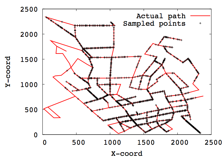
A more immediate visualization of the inaccuracy is given in the Figure below.
This figure shows, for the case of a node with a maximum uncovered interval
equal to 200s (i.e., locating this node in the lowest 10th percentile),
its real trajectory (the unbroken line), and the sample points the agent
collected.